Introduction to SQL (Microsoft SQL Server)
This is a very basic tutorial on how to access Microsoft SQL Server data via SQL queries. Since these are generic concepts, they will be applicable in most other SQL variants out there. My hope is that it will provide the necessary tools to quickly "get into it" without having to read (or understand) too much. Where you go from there is on you.
There are a lot of basic concepts about SQL, this post will be pretty long.
Table of contents
- Connecting to a database - how to use SQL Management Studio to access a database
- Getting data from tables - simple SELECT operations
- Defining tables and inserting data - CREATE TABLE and INSERT data
- Changing existing data - UPDATE and DELETE operations
- The NULL value - explaining the concept of NULL (value not set)
- Combining data from multiple sources - JOINs and UNIONs
- Indexes and relationships. Performance. - short intro to indexes
- When indexes are bad - indexes are good for reading, bad for writing
- Conclusion - thanks for reading
Connecting to a database
Let's start with tooling. To access a database you will need SQL Server Management Studio, in my case version 2022, but I will not do anything complicated with it here, therefore any version will do just fine. I will assume you have it installed already as installation is beyond the scope of the blog post. Starting it will prompt for a connection:
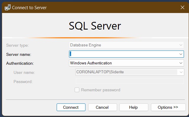 To connect to the local computer, the server will be either . or (local) or the computer name. You can of course connect to any server and you can specify the "instance" and the port number as well. An instance is a specific named installation of SQL server which allows one to have multiple installations (and even versions) of SQL Server. In fact, each instance has its own port, so specifying the port number will ignore the name of the instance. The default port is usually 1433.
Example of connection server strings: Computer1\SQLEXPRESS, sql.corporate.com,1433, (local), .
The image here is from a connection to the local machine using Windows Authentication (your windows user). You can connect using SQL Server Authentication, which means providing a username and a password, or using one of the more modern Azure Active Directory methods.
I will also assume that the connection parameters are known to you, so let's go to the next step.
Once connected, the Object Explorer window will display the connection you've opened.
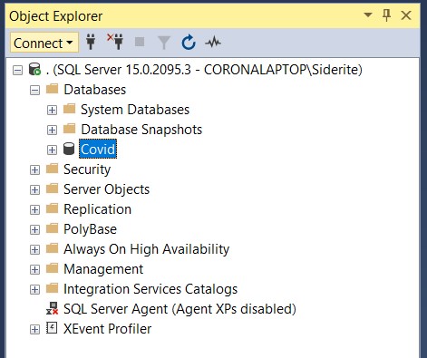 Expanding the Databases node will show the available databases.
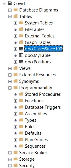 Expanding a database node we get the objects that are part of the database, the most important being:
- Tables - where the actual data resides
- Views - abstractions over more complex queries that behave like tables as much as possible, but with some restrictions
- Stored Procedures - SQL code that can be executed with parameters and may return data results
- Functions - SQL code that can be executed and returns a value (which can be scalar, like a number of string, or a table type, etc.)
In essence they are the equivalent of data stores and code that is executed to use those stores. Views, SPs and functions will not be explained in this post, but feel free to read about them afterwards.
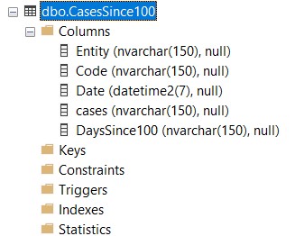 If one expands a table node, the child nodes will contains various things, the most important of which are:
- Columns - the names and types of each column in the table
- Indexes - data structures designed to increase performance to various ways of accessing the data in the table
- Constraints and Keys - logical restrictions and relationships between tables
Tables are kind of like Excel sheets, they have rows (data records) and columns (record properties). The power of SQL is a way to declare what you want from tabular representations of data and get the results quickly and efficiently.
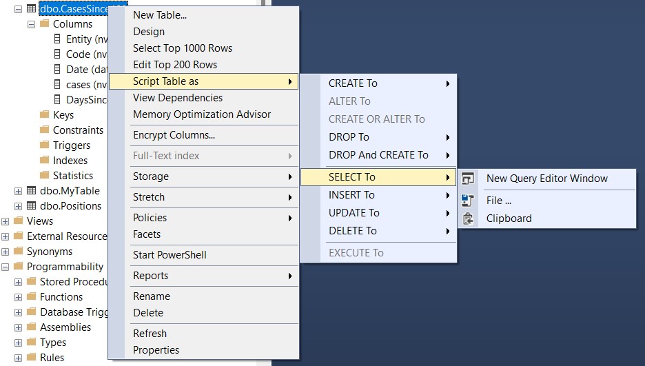 Last thing I want to show from the graphical interface is right clicking on a table node, which shows multiple options, including generating simple operations on the table, the CRUD (Create, Read, Update, Delete) operations mostly, which in SQL are called INSERT, SELECT, UPDATE and DELETE respectively.
The keywords are traditionally written in all caps, I am not shouting at you. Depending on your preferences and of course the coding standards that apply to your project you can capitalize SQL code however you like. SQL is case insensitive.
Anyway, whatever you are going to choose to "script" it's going to open a so called query window and show you a text with the query. You then have the option of executing it. Normally no one uses the UI to generate scripts except for getting the column names in order for SELECT or INSERT operations. Most of the time you will just right click on a database and choose New Query or select a database and press Ctrl-N, with the same result.
Getting data from tables
Finally we get to doing something. The operation to read data from SQL is called SELECT. One can specify the columns to be returned or just use * to get them all. It is good practice to always specify the column names in production code, even if you intend to select all columns, as the output of the query will not change if we add more columns in the future. However, we will not be discussing software projects, just how to get or change the data using SQL server, so let's get to it.
The simplest select query is: SELECT * FROM MyTable, which will return all columns of all records of the table. Note that MyTable is the name of a table and the least specific way of accessing that table. The same query can be written as: SELECT * FROM [MyDatabase].[dbo].[MyTable], specifying the database name, the schema name (default one is dbo, but your database can use multiple ones) and only then the table name.
The square bracket syntax is usually not required, but might be needed in special cases, like when a column has the same name as a keyword or if an object has spaces or commas in it (never a good idea, but a distinct possibility), for example: SELECT [Stupid,column] FROM [Stupid table name with spaces]. Here we are selecting a badly named column from a badly named table. Removing the square brackets would result in a syntax error.
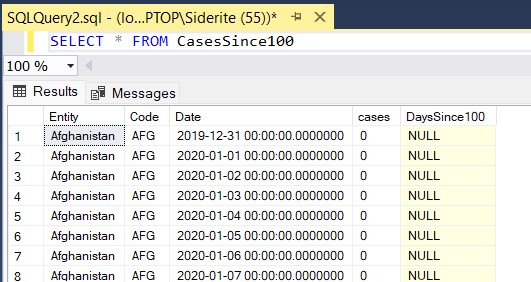
In the example above we selected stuff from table CasesSince100 and we got tabular results for every record and the columns defined in the table. But that is not really useful. What we want to do when getting data is:
- getting data from specific columns
- formatting the data for our purposes
- filtering the data on conditions
- grouping the data
- ordering the results
So here is a more complex query:
-- everything after two dashes in a line is a comment, ignored by the engine
/* there is also
a multiline comment syntax */
SELECT TOP 10 -- just the first 10 records
c.Entity as Country, -- Entity will be returned with the name Country
CAST(c.[Date] as Date) as [Date], -- Unfortunate naming, as Date is also a type
c.cases as Cases -- capitalized alias
FROM CasesSince100 c -- source for the data, aliased as 'c'
WHERE c.Code='ROU' -- conditions to filter by
AND c.[Date]>'2020-03-01'
ORDER BY c.[Date] DESC -- ordering in descending order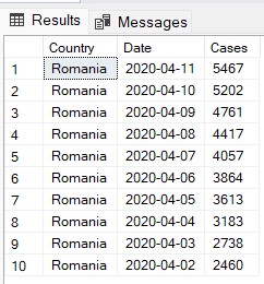 The query above will return at most 10 rows, only for Romania, for dates larger than March 2020, but ordered from the newest to oldest. Data returned will be the country name, the date (which was originally a DATETIME and now is cast to a timeless DATE type) and the number of cases.
Note that I have aliased all columns, so the resulting table has columns named as the aliases. I've also aliased the table name as 'c', which helps in several ways. First of all, Intellisense works better and faster when specifying the table name. All you have to do is type c. and the list of columns will pop up and be filtered as you type. The second reason will become apparent when I am talking about updating and deleting. For the moment just remember that it's a good idea to alias your tables.
You can alias a table by specifying a name to call it by next to its own name and optionally using 'as', like SELECT ltn.* FROM Schema.LongTableName as ltn. It helps differentiating between ambiguous names (like if two joined tables have columns with the same name), simplifying the code for long named tables and helping with code completion. Even when aliased, the table name can be used and one can specify or ignore the name of the table if the column names are unambiguous.
Of course these are trivial examples. The power of SQL is that you can get information from multiple sources, aggregate them and structure your database for quick access. More advanced concepts are JOINs and indexes, and I hope you will read until I get there, but for now let's just go through the very basics.
Here is another query that groups and aggregates data:
SELECT TOP 10 -- top 10 results
c.Entity as Country, -- country name
SUM(CAST(c.cases as INT)) as Cases -- cases is text, so we transform it to int
FROM CasesSince100 c
WHERE YEAR([Date])=2020 -- condition applies a function to the date
GROUP BY c.Entity -- groups by country
HAVING SUM(CAST(c.cases as INT))<1000000 -- this is filtering on grouped values
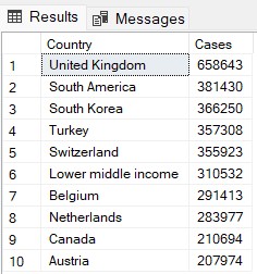
ORDER BY SUM(CAST(c.cases as INT)) DESC -- order on sum of casesThis query will show us the top 10 countries and the total sum of cases in year 2020, but only for countries where that total is less than a million. There is a lot to unpack here:
- cases column is declared as NVARCHAR(150) meaning Unicode strings of varied length, but at most 150 characters, so we need to cast it to INT (integer) to be able to apply summing to it
- there are two different ways of filtering: WHERE, which applies to the data before grouping, then HAVING, which applies to data after grouping
- filtering, grouping, ordering all work with unaliased columns, so even if Entity is returned as Country, I cannot do
WHERE Country='Romania' - grouping allows to get a row for each combination of the columns the grouping is done and compute some sort of aggregation (in the case above, a sum of cases per country)
Here are the results:
Let me rewrite this in a way that is more readable using what is called a subquery, in other words a query from which I will query once again:
SELECT TOP 10
    Country,
	SUM(Cases) as Cases
FROM (
    SELECT
        c.Entity as Country,
        CAST(c.cases as INT) as Cases,
	    YEAR([Date]) as [Year]
FROM CasesSince100 c
) x
WHERE [Year]=2020
GROUP BY Country
HAVING SUM(Cases)<1000000
ORDER BY Cases DESC
Note that I still have to use SUM(Cases) in the HAVING clause. I could have grouped it in another subquery and selected again and so on. In order to select from a subquery, you need to name it (in our case, we named it x). Also I selected Country from x, which I could have also written as x.Country. As I said before, table names (aliased or not) are optional if the column name if unambiguous. Also you may notice that I've given a name to the summed column. I could have skipped that, but that would mean the resulting columns would have had no name and the query itself would have been difficult to use in code (extracted column values would have had to be retrieved by index and not by name, which is never recommended).
If you think about it, the order of the clauses in a SELECT operation has a major flaw: you are supposed to write SELECT, then specify what columns you want and only then specify where you want the columns to be read from. This makes code completion problematic, which is why the in code query language for .NET (LInQ) puts the selection at the end. But even so there is a trick:
- SELECT * and then complete the query
- go back and replace the * with the column names you want to extract (you will now have Intellisense code completion)
- the alias of the tables will now come in handy, but even without aliases one can press Ctrl-Space and get a list of possible values to select
Defining tables and inserting data
Before we start inserting information, let's create a table:
CREATE TABLE Food(
    Id INT IDENTITY(1,1) PRIMARY KEY,
    FoodName NVARCHAR(100),
    Quantity INT
)
One important concept in SQL is the primary key. It is a good idea in most cases that your tables have a primary key which identifies each record uniquely and also makes them easy to reference. Let me give you an example. Let's assume that we would put no Id column in our Food table and then we would accidentally add cheese twice. How would you reference the first record as opposed to the second? How would you delete the second one?
A primary key is actually just a special case of a unique index, clustered by default. We will get to indexes later, so don't worry about that yet. Enough to remember that it is fastest (most efficient) to find records by the primary key than any other column combination and the way records are uniquely identified.
The IDENTITY(1,1) notation tells SQL Server that we will not insert values in that column and instead let it put values starting with 1, then increasing with 1 each time. That functionality will become clear when we INSERT data in the table:
INSERT INTO Food(FoodName,Quantity)
VALUES('Bread',1),('Cheese',1),('Pork',2),('Chilly',10)
Selecting from our Food table now gets us these results:
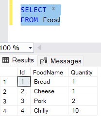
As you can see, we've inserted four records, by only specifying two out of three columns - we skipped Id. Yet SQL has filled the column with values from 1 to 4, starting with 1 and incrementing each time with 1.
The VALUES syntax is specifying inline data, but we could, in fact, insert into a table the results of a query, something like this:
INSERT INTO Food(FoodName,Quantity)
SELECT [Name],Quantity
FROM Store
WHERE [Type]='Food'
There is another syntax for insert that is useful with what are called temporary tables, tables created for the purpose of your session (lifetime of the query window) and that will automatically disappear once the session is over. It looks like this:
SELECT FoodName,Quantity
INTO #temp
FROM Food
This will create a table (temporary because of the # sign in front of it) that will have just FoodName and Quantity as columns, then proceed on saving the data there. This table will not have a primary key nor any types of indexes and it will work as a simple dump of the data selected. You can add indexes later or alter the table in any way you want, it works just like a regular table. While a convenient syntax (you don't have to write a CREATE TABLE query or think of the type of columns) it has a limited usefulness and I recommend not using it in application code.
Just as one creates a table, there are DROP TABLE and ALTER TABLE statements that delete or change the structure of the table, but we won't go into that.
Changing existing data
So now we have some data in a table that we have defined. We will see how the alias syntax I discussed in the SELECT section will come in handy. In short, I propose you use just two basic syntax forms for all CRUD operations: one for INSERT and one for SELECT, UPDATE and DELETE.
But how can you use the same syntax for statements that are so different, I hear you ask? Let me give you some example of similar code doing just that before I dive in what each operation does.
SELECT *
FROM Food f
WHERE f.Id=4

UPDATE f
SET f.Quantity=9
FROM Food f
WHERE f.Id=4

DELETE FROM f
FROM Food f
WHERE f.Id=4
The last two lines of all operations are exactly the same. These are simple queries, but imagine you have a complex one to craft. The first thing you want to see is that you are updating or deleting the right thing, therefore it makes sense to start with a SELECT query instead, then change it to a DELETE or UPDATE when satisfied. You see I UPDATE and DELETE using the alias I gave the table.
When first learning UPDATE and DELETE statements, one usually gets to this syntax:
UPDATE Food     -- using the table name is cumbersome if in a complex query
SET Quantity=9  -- unless using Food.Quantity and Food.Id
WHERE Id=4      -- you don't get easy Intellisense

DELETE          -- this seems a lot easier to remember
FROM Food       -- but it only works with one table in a simple query
WHERE Id=4
I've outlined some of the reasons I don't use this syntax in the comments, but the most important reason why one shouldn't use them except for very simplistic cases is that you are trying to create a query to destructively change the data in the database and there is no fool proof way to duplicate the same logic in a SELECT query to verify what you are going to change. I've seen people (read that as: I was dumb enough to do it myself) who created an entire different SELECT statement to verify what they would do, then realize to their horror the statements were not equivalent and they had updated or deleted the wrong thing!
OK, let's look at UPDATE and DELETE a little closer.
One of the useful clauses for these statements is, just like with SELECT, the TOP clause, which instructs SQL to affect just a finite number of rows. However, because TOP has been added later for write operations, you need to encase the value (or variable) in parentheses. For SELECT you can skip the parentheses for constant values (you still need them for variables)
DELETE TOP (10) FROM MyTableAnother interesting clause, that frankly I have not used a lot, but is essential in some specific cases, is OUTPUT. One can delete or update some rows and at the same time get the rows they have changed. The reason being that first of all in a DELETE statement the rows will be gone, so you won't be able to SELECT them again. But even in an UPDATE operation, the rows chosen to be updated by a query may not be the same if you execute them again.
SQL does not guarantee the order of rows unless specifically using ORDER BY. So if you execute SELECT TOP 10 * FROM MyTable twice, you may get two different results. Moreover, between the time you UPDATE some rows and you SELECT them in another query, things may change because of other processes running at the same time on the same data.
So let's say we have some for of Invoices and Items tables that reference each other. You want to delete one invoice and all the items associated with it. There is no way of telling SQL to DELETE from multiple tables at the same time, so you DELETE the invoice, OUTPUT its Id, then delete the items for that Id.
CREATE TABLE #deleted(Id INT) -- temporary table, but explicitly created

DELETE FROM Invoice
OUTPUT Deleted.Id    -- here Deleted is a keyword
INTO #deleted        -- the Id from the deleted rows will be stored here
WHERE Id=2           -- and can be even be restored from there

DELETE
FROM Item
WHERE Id IN (
  SELECT Id FROM #deleted
)  -- a subquery used in a DELETE statement

-- same thing can be written as:
DELETE FROM i
FROM Item i
INNER JOIN #deleted d  -- I will get to JOINs soon
ON i.Id=d.Id
I have been informed that the INTO syntax is confusing and indeed it is:
- SELECTing INTO will create a new table with results and throw an exception if the table already exists. The table will have the names and types of the selected values, which may be what one wants for a quick data dump, but it may also cause issues. For example the following query would throw an exception:
SELECT 'Blog' as [Name] INTO #temp INSERT INTO #temp([Name]) -- String or binary data would be truncated error VALUES('Siderite') because the Name column of the new temporary table would be VARCHAR(4), just like 'Blog' and 'Siderite' would be too long
- UPDATEing or DELETEing with OUTPUT INTO will require an existing table with the same number and types of columns as the columns specified in the OUTPUT clause and will throw an exception if it doesn't exist
One can use derived values in UPDATE statements, not just constants. One can reference the columns already existing or use any type of function that would be allowed in a similar SELECT statement. For example, here is a query to get the tax value of each row and the equivalent update to store it into a separate column:
SELECT
    i.Price,
    i.TaxPercent,
    i.Price*(i.TaxPercent/100) as Tax  -- best practice: SELECT first
FROM Item i

UPDATE i
SET Tax = i.Price*(i.TaxPercent/100)   -- UPDATE next
FROM Item i
So here we first do a SELECT, to see if the values we have and calculate are correct and, if satisfied, we UPDATE using the same logic. Always SELECT before you change data, so you know you are changing the right thing.
There is another trick to help you work safely, one that works on small volumes of data, which involves transactions. Transactions are atomic operations (all or nothing) which are defined by starting them with BEGIN TRANSACTION and are finalized with either COMMIT TRANSACTION (save the changes to the database) or ROLLBACK TRANSACTION (revert changes to the database). Transactions are an advanced concept also, so read about it yourself, but remember one can do the following:
- open a new query window
- execute BEGIN TRANSACTION
- do almost anything in the query window
- if satisfied with the result execute COMMIT TRANSACTION
- if any issue with what you've done execute ROLLBACK TRANSACTION to undo the changes
Note that this only applies for stuff you do in that query window. Also, all of these operations are being saved in the log of the database, so this works only with small amounts of data. Attempting to do this with large amounts of data will practically duplicate it on disk and take a long time to execute and revert.
The NULL value
We need a quick primer on what NULL is. NULL is a placeholder for a value that was not set or is considered unknown. It's a non-value. It is similar to null in C# or JavaScript, but with some significant differences applicable to SQL only. For example, a NULL value (an oxymoron for sure) will never be equal to (or not equal to) or less than or greater than anything. One might expect to get all the values in a table in these two queries: SELECT * FROM MyTable WHERE Value>5 and SELECT * FROM MyTable WHERE Value<=5. But if any rows will have NULL for a Value, then they will not appear in any of the query results. That applies to the negation operator NOT as well: SELECT * FROM MyTable WHERE NOT (Value>5).
This behavior can be changed by using SET ANSI_NULLS OFF, but I am yet to see a database that has ever been set up like this.
To check if a value is or is not NULL, one uses the IS and IS NOT syntax :)
SELECT *
FROM MyTable
WHERE MyValue IS NOT NULL
The NULL concept will be used a lot in the next chapter.
Combining data from multiple sources
We finally go to JOIN operations. In most scenarios, you have a database containing multiple table, with intricate connections between them. Invoices that have items, customers, the employee that processed it, dates, departments, store quantities, etc., all referencing something. Integrating data from multiple tables is a complex subject, but I will touch just the most common and important parts:
- INNER JOIN
- OUTER JOIN
- EXISTS
- UNION / UNION ALL
Let's write a query that displays the name of employees and their department. I will show the CREATE TABLE statements, too, in order to see where we get the data from:
CREATE TABLE Employee (
  EmployeeId INT,          -- Best practice: descriptive column names
  FirstName NVARCHAR(100),
  LastName NVARCHAR(100),
  DepartmentId INT)        -- Best practice: use same name for the same thing

CREATE TABLE Department (
  DepartmentId INT,        -- same thing here
  DepartmentName NVARCHAR(100)
)

SELECT
    CONCAT(FirstName,' ',LastName) as Employee,
    DepartmentName
FROM Employee e
INNER JOIN Department d
ON e.DepartmentId=d.DepartmentId
Here it is: INNER JOIN, a clause that combines the data from two tables based ON a condition or series of conditions. For each row of Employee we are looking for the corresponding row of Department. In this example, one employee belongs to only one department, but a department can hold multiple employees. It's what we call a "one to many relationship". One can have "one to one" or "many to many" relationships as well. That is very important when trying to gauge performance (and number of returned rows).
Our query will only find at most one department for each employee, so for 10 employees we will get at most 10 rows of data. Why do I say "at most"? Because the DepartmentId for some employees might not have a corresponding department row in the Department table. INNER JOIN will not generate records if there is no match. But what if I want to see all employees, regardless if their department exists or not? Then we use an OUTER JOIN:
SELECT
    CONCAT(FirstName,' ',LastName) as Employee,
    DepartmentName
FROM Employee e
LEFT OUTER JOIN Department d
ON e.DepartmentId=d.DepartmentId
This will generate results for each Employee and their Department, but show a NULL (without value) result if the department does not exist. In this case LEFT is used to define that there will be rows for each record in the left table (Employee). We could have used RIGHT, in which case we would have rows for each department and NULL values for departments that have no employees. There is also the FULL OUTER JOIN option, in which case we will get both departments with NULL employees if none are attached and employees with NULL departments in case the department does not exist (or the employee is not assigned - DepartmentId is NULL)
Note that the keywords INNER and OUTER are completely optional. JOIN is the same thing as INNER JOIN and LEFT JOIN is the same as LEFT OUTER JOIN. I find that specifying them makes the code more readable, but that's a personal choice.
The OUTER JOINs are sometimes used in a non intuitive way to find records that have no match in another table. Here is a query that shows employees that are not assigned to a department:
SELECT
    CONCAT(FirstName,' ',LastName) as Employee
FROM Employee e
LEFT OUTER JOIN Department d
ON e.DepartmentId=d.DepartmentId
WHERE d.DepartmentId IS NULL
Until now, we talked about the WHERE clause as a filter that is applied first (before grouping) so one might intuitively have assumed that the WHERE clauses are applied immediately on the tables we get the data from. If that were the case, then this query would never return anything, because every Department will have a DepartmentId. Instead, what happens here is the tables are LEFT JOINed, then the WHERE clause applies next. In the case of unassigned employees, the department id or name will be NULL, so that is what we are filtering on.
So what happens above is:
- the Employee table is LEFT JOINed with the Department table
- for each employee (left) there will be rows that contain the values of the Employee table rows and the values of any matched Department table rows
- in the case there is no match, NULL values will be returned for the Department table for all columns
- when we filter by Department.DepartmentId being NULL we don't mean any Department that doesn't have an Id (which is impossible) but any Employee row with no matching Department row, which will have a NULL value where the Department.DepartmentId value would have been in case of a match.
- not matching can happen for two reasons: Employee.DepartmentId is NULL (meaning the employee has not been assigned to a department) or the value stored there has no associated Department (the department may have been removed for some reason)
Also, note that if we are joining tables on some condition we have to be extra careful with NULL values. Here is how one would join two tables on VARCHAR columns being equal even when NULL:
SELECT *
FROM Table1 t1
INNER JOIN Table2 t2
ON (t1.Value IS NULL AND t2.Value IS NULL) OR t1.Value=t2.Value

SELECT *
FROM Table1 t1
INNER JOIN Table2 t2
ON ISNULL(t1.Value,'')=ISNULL(t2.Value,'')
The second syntax seems promising, doesn't it? It is more readable for sure. Unfortunately, it introduces some assumptions and also decreases the performance of the query (we will talk about performance later on). The assumption is that if Value is an empty string, then it's the same as having no value (being NULL). One could use something like ISNULL(Value,'--NULL--') but now it starts looking worse.
There are other ways of joining two tables (or queries, or table variables, or table functions, etc.), for example by using the IN or the EXISTS/NOT EXISTS clauses or subqueries. Here are some examples:
SELECT *
FROM Table1
WHERE MyValue IN (SELECT MyValue FROM Table2)

SELECT *
FROM Table1
WHERE MyValue = (SELECT TOP 1 MyValue FROM Table2 WHERE Table1.MyValue=Table2.MyValue)

SELECT *
FROM Table1
WHERE NOT EXISTS(SELECT * FROM Table2 WHERE Table1.MyValue=Table2.MyValue)
These are less readable, usually have terrible performance and may not return what you expect them to return.
When I was learning SQL, I thought using a JOIN would be optimal on all cases and subqueries in the WHERE clause were all bad, no exception. That is, in fact, false. There is a specific case where it is better to use a subquery in WHERE instead of JOIN, and that is when trying to find records that have at least one match. It is better to use EXISTS because it is short-circuiting logic which leads to better performance.
Here is an example with different syntax for achieving the same goal:
SELECT DISTINCT d.DepartmentId
FROM Department d
INNER JOIN Employee e
ON e.DepartmentId=d.DepartmentId

SELECT d.DepartmentId
FROM Department d
WHERE EXISTS(SELECT * FROM Employee e WHERE e.DepartmentId=d.DepartmentId)
Here, the search for departments with employees will return the same thing, but in the first situation it will get all employees for all departments, then list the department ids that had employees, while in the second query the department will be returned the moment just one employee that matches is found.
There is another way of combining data from two sources and that is to UNION two or multiple result sets. It is the equivalent of taking rows from multiple sources of the same type and showing them together in the same result set.
Here is a dummy example:
SELECT 1 as Id
UNION
SELECT 2
UNION
SELECT 2
And we execute it and...
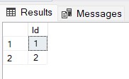
What happened? Shouldn't there have been three values? Somehow, when copy pasting the silly example, you added two identical values. UNION will add only distinct values to the result set. using UNION ALL will show all three values.
SELECT 1 as Id
UNION ALL
SELECT 2
UNION ALL
SELECT 2

SELECT DISTINCT Id FROM (
  SELECT 1 as Id
  UNION ALL
  SELECT 2
  UNION ALL
  SELECT 2
) x
The first query will return 1,2,2 and the second will be the equivalent of the UNION one, returning 1 and 2. Note the DISTINCT keyword.
My recommendation is to never use UNION and instead use UNION ALL everywhere, unless it makes some kind of sense for a very specific scenario, because the operation to DISTINCT values is expensive, especially for many and/or large columns. When results are supposed to be different anyway, UNION and UNION ALL will return the same output, but UNION is going to perform one more pointless distinct operation.
After learning about JOIN, my request to start with SELECT queries and only them modify them to be UPDATE or DELETE begins to make more sense. Take a look at this query:
UPDATE d
SET ToFindManager=1
--SELECT *
FROM Department d
LEFT OUTER JOIN Employee e
ON d.DepartmentId=e.DepartmentId
AND e.[Role]='Manager'
WHERE e.EmployeeId IS NULL
This will set ToFindManager in departments that have no corresponding manager. But if you select the text from SELECT * on and then execute, you will get the results that you are going to update. Same query, executing by selecting different sections of it will either verify or perform the operation.
Indexes and relationships. Performance.
We have seen how to define tables, how to insert, select, update and delete records from them. We've also seen how to integrate data from multiple sources to get what we want. The SQL engine will take our queries, try to understand what we meant, optimize the execution, then give us the results. However, with large enough data, no amount of query optimization will help if the relationships between tables are not properly defined and tables are not prepared for the kind of queries we will execute.
This requires an introduction to indexes, which is a rather advanced idea, both in terms of how to create, use, debug and profile, but also as a computer science concept. I will try to stick to the basics here, and you go and get more in depth from here.
What is an index? It's a separate data structure that will allow quick access to specific parts of the original data. A table of contents in a blog post is an index. It allows you to quickly jump to the section of the post without having to read it all. There are many types of indexes and they are used in different ways.
We've talked about the primary key: (unless specified differently) it's a CLUSTERED, UNIQUE index. It can be on a single column or a combination of columns. Normally, the primary key will be the preferred way to find or join records on, as it physically rearranges the table records in order and insures only one record has a particular primary key.
The difference between CLUSTERED and NONCLUSTERED indexes is that a table can have only one clustered index, which will determine the physical order of record data on the disk. As an example, let's consider a simple table with a single integer column called X. If there is a clustered index on X, then when inserting new values, data will be moved around on the disk to account for this:
CREATE TABLE Test(X INT PRIMARY KEY)

INSERT INTO Test VALUES (10),(1),(20)

INSERT INTO Test VALUES (2),(3)

DELETE FROM Test WHERE X=1
After inserting 10,1 and 20, data on the disk will be in the order of X: a 1, followed by a 10, then a 20. When we insert values 2 and 3, 10 and 20 will have to be moved so that 2 and 3 are inserted. Then, after deleting 1, all data will be moved so that the final physical order of the data (the actual file on the disk holding the database data) will be 2,3,10,20. This will help optimize not only finding the rows, but also efficiently reading them from disk (disk access is the most expensive operation for a database).
Note: deletion is working a little differently in reality, but in theory this is how it would work.
Nonclustered indexes, on the other hand, keep their own order and reference the records from the original data. For such a simple example as above, the result would be almost identical, but imagine you have the Employee table and you create a nonclustered index on LastName. This means that behind the scenes, a data structure that looks like a table is created, which is ordered by LastName and contains another column for EmployeeId (which is the primary key, the identifier of an employee). When you do SELECT * FROM Employee ORDER BY LastName, the index will be used to first get a list of ids, then select the values from them.
A UNIQUE index also insures that no two records will have the same combination of values as defined therein. In the case of the primary key, there cannot be two records with the same id. But one can imagine something like:
CREATE UNIQUE INDEX IX_Employee_Name ON Employee(FirstName,LastName)

INSERT INTO Employee (FirstName,LastName)
VALUES('Siderite','Blog')
IX_Employee_Name is a nonclustered unique index on FirstName and LastName. If you execute the insert, it will work the first time, but fail the second time:
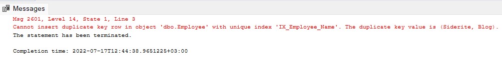
There is another type of index-like structure called a foreign key. It should be used to define logical relationships between tables. For the Department table, DepartmentId should be a primary key, but in the Employee table, DepartmentId should be defined as a foreign key connecting to the column in the Department table.
Important note: a foreign key defines the relationship, but doesn't index the column. A separate index should be added on the Employee.DepartmentId column for performance reasons.
I don't want to get into foreign keys here. Suffice to say that once this relationship is defined, some things can be achieved automatically, like deleting corresponding Item records by the engine when deleting Invoices. Also the performance of JOIN queries increases.
Indexes can be used not only on equality, but also other more complex cases: numerical ranges, prefixes, etc. It is important to understand how they are structured, so you know when to use them.
Let's consider the IX_Employee_Name index. The index is practically creating a tree structure on the concatenation of the first and last name of the employee and stores the primary key columns for the table for reference. It will work great for increasing performance of a query like SELECT * FROM Employee ORDER BY FirstName or SELECT * FROM Employee WHERE FirstName LIKE 'Sid%'. However it will not work for LastName queries or contains queries like SELECT * FROM Employee ORDER BY LastName or SELECT * FROM Employee WHERE FirstName LIKE '%derit%'.
That's important because sometimes simpler queries will take more resources than more complicated ones. Here is a dumb example:
CREATE INDEX IX_Employee_Dumb ON Employee(
    FirstName,
    DepartmentId,
    LastName
)

SELECT *
FROM Employee e
WHERE e.FirstName='Siderite'
  AND e.LastName='Blog'

SELECT *
FROM Employee e
WHERE e.FirstName='Siderite'
  AND e.LastName='Blog'
  AND e.DepartmentId=1
The index we create is called IX_Employee_Dumb and it creates a data structure to help find rows by FirstName, DepartmentId and LastName in that order.
For some reason, in our employee table there are a lot of people called Siderite, but with different departments and last names. The first query will use the index to find all Siderite employees (fast), then look into each and check if LastName is 'Blog' (slow). The second query will directly find the Siderite Blog employee from department with id 1 (fast), because it uses all columns in the index. As you can see, the order of columns in the index is important, because without the DepartmentId in the WHERE clause, only the first part of the index, for FirstName, can be used. In the last query, because we specify all columns, the entire index can be used to efficiently locate the matching rows.
Note 2022-09-06: Partitioning a table (advanced concept) takes precedence to indexes. I had a situation where a table was partitioned on column RowDate into 63 partitions. The primary key was RowId, but when you SELECTed on RowId, there were 63 index seeks performed. If queried on RowId AND RowDate, it went to the containing partition and did only one index seek inside it. So careful with partitioning. It only provides a benefit if you query on the columns you use to partition on.
One more way of optimizing queries is using the INCLUDE clause. Imagine that Employee is a table with a lot of columns. On the disk, each record is taking a lot of space. Now, we want to optimize the way we get just FirstName and LastName when searching in a department:
SELECT FirstName,LastName
FROM Employee
WHERE DepartmentId=@departmentId
That @ syntax is used for variables and parameters. As a general rule, any values you send to an SQL query should be parameterized. So don't do in C# var sql = "SELECT * FROM MyTable WHERE Id="+id, instead do var sql="SELECT * FROM MyTable WHERE Id=@id" and add an @id parameter when running the query.
So, in the query above SQL will do the following:
- use an index for DepartmentId if any (fast)
- find the EmployeeId
- read the (large) records of each employee from the table (slow)
- extract and return the first and last name for each
But add this index and there is no need to even go to the table:
CREATE INDEX IX_Employee_DepWithNames
  ON Employee(DepartmentId)
  INCLUDE(FirstName,LastName)
What this will do is add the values of FirstName and LastName to the data inside the index and, if only selecting values from the include list, return them from the index directly, without having to read records from the initial table.
Note that DepartmentId is used to locate rows (in WHERE and JOIN ON clauses) while FirstName and LastName are the columns one SELECTs.
Indexes are a very complex concept and I invite you to examine it at length. It might even be fun.
When indexes are bad
Before I close, let me tell you where indexes are NOT recommended.
One might think that adding an index for each type of query would be a good thing and in some scenarios it might, but as usual in database work, it depends. What performance you gain for finding records in SELECT, UPDATE and DELETE statements, you lose with INSERT, UPDATE and DELETE data changes.
As I explained before, indexes are basically hidden tables themselves. Slight differences, but the data they contain is similar, organized in columns. Whenever you change or add data, these indexes will have to be updated, too. It's like writing in multiple tables at the same time and it affects not only the execution time, but also the disk space.
In my opinion, the index and table structure of a database depends the most on if you intend to read a lot from it or write a lot to it. And of course, everybody will scowl and say: "I want both! High performance read and write". My recommendation is to separate the two cases as much as possible.
- You want to insert a lot of data and often? Use large tables with many columns and no indexes, not even primary keys sometimes.
- You want to update a lot of data and often? Use the same tables to insert the modifications you want to perform.
- You want to read a lot of data and often? Use small read only tables, well defined, normalized data, clear relationships between tables, a lot of indexes
- Have a background process to get inserts and updates and translate them into read only records
Writing data and reading data, from the SQL engine perspective, are very very different things. They might as well be different software and indeed some companies use one technology to insert data (like NoSQL databases) and another to read it.
Conclusion
I hope the post hasn't been too long and that it will help you when beginning with SQL. Please leave any feedback that you might have, the purpose of this blog is to help people and every perspective helps.
SQL is a very interesting idea and has changed the way people think of data access. However, it has become so complex that most people are still confused even after years of working with it. Every year new features are being added and new ideas are put forward. Yet there are a few concepts, a foundation if you will, that will get you most of the way there. This is what I have tried to distil here. Hope I succeeded.
Comments
You are welcome! I would be grateful for any feedback.
Sideriteas an SQL beginner this was very informative thank you!
Hasmidr